What is Entropy? Every system tends toward equilibrium or a steady state, conserving energy while maximizing entropy. Entropy is a scientific thermodynamic measure (of the universe, system, or control volume) that can increase with time because it is mostly a consequence of rearranging energy and distributing it (often more uniformly). While it is most commonly described as a “measure of disorder or randomness,” it is more precisely defined as a measure of how many different ways a system and its energy can rearrange itself within its constraints. The engineering symbol for entropy is S, with units of joules per kelvin (J/K). Or the lowercase “s,” which is the entropy per unit volume or per mole.
Entropy is a thermodynamic state variable that quantifies the probability distribution of energy and mass over a system’s accessible microstates. This definition describes the entropy as being proportional to the natural logarithm of the number of possible microscopic configurations of the individual atoms and molecules of the system (microstates) that could cause the observed macroscopic state (macrostate) of the system. The constant of proportionality is the Boltzmann constant.
The classical definition of entropy, which we commonly use in engineering calculations, is that the entropy change, dS, of a system that is undergoing a reversible process (with changes in the state-defining variables) is equal to the reversible heat transfer (dQrev) divided by the temperature, T, in Kelvin. dS = dQrev/T. Thermodynamic variables are precise, and a collection of them (for example, pressure, temperature, and chemical potential) describes the state of a system (meaning they can be used to infer other thermodynamic variables); a system can transition between thermodynamic states along a reversible or irreversible path.
Reversible paths do not require entropy production; irreversible paths imply entropy production/generation (EG). It turns out that when entropy is generated, it is associated with a rate of generation
What is Entropy Generation Rate (EGR) and why is it important? When energy is transferred, rearranged, or used for an objective, new entropy is always created (effectively, we are saying that reversibility is never experienced). This new entropy production is called entropy generation from the process. What happens to this new entropy, and how it is produced, is fundamentally important to transformation efficiency and the residual useful patterns that result. We would not have thought much about Black Holes without invoking entropy generation. In the 1970s, physicists Bekenstein and Hawking shocked the scientific world by defining black holes not just as dead stars, but as thermodynamic objects that possess and generate massive amounts of entropy.
What Events Generate Entropy: Gradients in anything especially temperature, chemical potential, pressure will generate entropy. Unrestrained expansion generates entropy, as does mixing and friction/viscous dissipation. All spontaneous reactions generate entropy. In fact when thinking about the rate of entropy generation it is useful as we will see below to speak about the rate of entropy generation per unit volume or per mole as the key measure.
Entropy generation invariably reduces traditional thermodynamic efficiencies of work output and also thermal power output. Regardless, it can be used in several creative ways for energy storage and other useful purposes, e.g., creating resilience to cracks and dislocations and other important properties. Entropy generation can produce beautiful patterns from Anti-Work, discussed below. Anti-Work underpins observable patterns in a self-organizing system. A self-organizing system is one in which the entropy generation rate clearly influences the transformation.
New entropy generation (production) results from gradients in temperature, pressure, chemical potential, electrical charge, or surfaces that manifest during a process. Such gradients are a result of temperature or pressure differences, reaction-prone chemical species aggregation, ionization, voltage differences, or phase-change reactions and similar processes, i.e., driven by thermodynamic forces, i.e., imbalances. Whenever a gradient exists, Onsager showed that new entropy is generated. The rate at which new entropy is generated (produced) is called the entropy generation rate (EGR). Unlike energy, entropy is not a conserved quantity, so this newly produced entropy adds to the overall entropy of the universe.
The discovery of entropy as a thermodynamic quantity arose from the critical understanding that led to the articulation of the Second Law of thermodynamics: the unavailability of part of a system’s thermal energy for conversion into work, often interpreted as the degree of disorder or randomness in the system (natural inherent randomness, which we will see further below, is an important feature of everything). The rate of entropy generation may be even more fundamental. Because energy conservation follows from local time-symmetry conditions, and energy itself could be a property of ripples in space-time, one definition of entropy is that it is merely a logarithmic measure of the rate at which information can be accurately transmitted in a particular message or language. When multiplied by the Boltzmann constant, this kind of rendering of the property-entropy yields dimensions (units) of entropy. The Boltzmann constant (k or kB) is a fundamental physical constant that links the average kinetic energy of particles in a gas to the temperature of that system. Its exactly defined value is 1.380649 × 10⁻²³ J K⁻ (the same as 1.380649 × 10⁻²³ m2 kg s-2 K-1). When multiplied by Avogadro’s number, the Boltzmann constant becomes the universal molar gas constant R, which has an exactly defined value of 8.3144 J mol-1 K-1.
The manifestations of work and heat rates are always practically apparent, but the manifestation of the entropy generation rate as a fundamentally important property is less so. Classical thermodynamics recognizes distinct pathways of work and heat for a change of state. Still, it stops short of describing how the rates of work and heat production (also known as useful power and heating rate, respectively) affect thermodynamically describable events. Classical thermodynamics thus does not easily address the entropy generation rate. As we will see below a knowledge of the entropy generation rate leads us to understand the changes in resilience and the connectivity during and after a process and thus allows us to examine the bridges (continuity and and boundaries) reshaped by Anti-Work and Anti-Power. In effect things don’t fall apart because of the nature of Anti-work!
The symbol for the entropy generation rate is:

which can only be zero (indicating equilibrium) or positive (indicating transitions).
The units are joules per kelvin per second (J/K·s). To isolate the specific mechanisms for entropy generation, the first law of thermodynamics (energy balance) and the second law of thermodynamics (entropy balance) can be combined.

U, T, S, P, and V denote internal energy, temperature, entropy, pressure, and volume. Yl represents intensive variables (such as mechanical stress, voltage, or chemical potential), and Xl represents their conjugate extensive parameters (strain, charge, or molar species). For an open control volume (subscript CV) operating at steady state, the rate of internal entropy generation is a function of driving gradients, where the subscripts CV and e stand for control volume and equilibrium exchange, respectively. When considering expansion, chemical transitions, and structural defects, the combined expression for an evolving system includes conjugate flux-force parameters. T
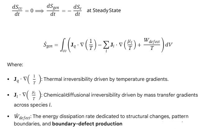
Although the equations above may look dauting they are similar to saying that the entropy change per mole between two states is the Boltzmann constant multiplied the Avogadro number (or moles multiplied by the gas constant) multiplied by R ln(V₂/V₁) when there is volume change, where V is the volume and 1 and 2 are the initial state and final state.
Similarly when unlike elements (say different chemical species) are mixed well and “perfectly” in a random configuration the entropy generation per mole is −R Σ xi ln xi where x is the mole fraction of the ith species.
If you think about it, once all the gradients have evened out, a new specific heat of the control volume or object is established. In this manner classical thermodynamics is able to account for final states but could miss some fundamental key processes that are in play because it fails to account for the Anti-power. These can include boundary defects such as dislocations, grain boundaries, and wear debris or electromagnetic phenomena. Defect can be equilibrium or non equilibrium type and distributed in a segregated manner..

Patterns are related to the entropy generation rate. Patterns have repetitive features, e.g., spacings, that influence engineering properties, such as resilience. For example, grain patterns influence the measured engineering hardness in crystallized metallic solids. A lower grain diameter commonly indicates a higher hardness. A higher rate of entropy production yields a finer pattern. To form a pattern, the system selects based on a principle called MEPR, discussed below. Pattern formation is linked to the rate of entropy generation, especially in steady-state open systems. Weather selection and cloud-type formation (patterns) are related to the rate of tropospheric entropy generation. A steady-state entropy generation rate can also be applied to bird flight formation assessments where entropy generation leads to stored work potential.
The importance of the rate of entropy generation (EGR) lies in two key practical aspects, namely, (i) it is related to the loss of efficiency in power-producing systems and (ii) it is related to pattern spacings and thus to contextual properties like resilience and connectivity. By analyzing EGR for a process, engineers can better design systems to minimize high-quality energy waste and predict long-term connectivity for environmental and mechanical stability. Source (link).
Most high-efficiency applications preserve energy quality.
The distribution of newly produced entropy and the overall energy across compartments depends on the process. Rapid processes typically create gradients (which is why conventional thermodynamics assumes slow change). A flux and a conjugate force generate entropy. For example, a heat (energy) flux is driven by a temperature gradient (the conjugate force) and thus creates new entropy (an example of Onsager’s relationship). In the picture below, new entropy is produced by thermal energy (heat) flowing down a temperature gradient in a metal rod held between two reservoirs at temperatures T1 and T0. This is a simple example that shows the entropy generation rate is maximized for several processes- see the article.
Are you wondering what patterns could be related to solid-state heat transfer? In metals, or at least when solids are near their melting points, heat transfer can cause noticeable atomic diffusion. Atoms migrate from hotter (higher-stress) regions to cooler regions along the boundaries between crystalline grains, which themselves respond to thermal conditions. This bulk atomic movement is a microscopic analog of fluid convection. In some solids, electron motion and related patterns can be driven by thermal gradients, and vice versa.

Entropy generation rate (Sgen rate) by heat transfer between two temperatures connected by a metal rod of length L. The direct power (rate of work) extracted, Pmax (J/s), is zero in this configuration.
Why is the concept of Maximum Entropy Generation Rate (MEPR) important? The Maximum Entropy Generation Rate (MEPR) principle – also sometimes referred to as the Maximum Entropy Production Principle (MEPP) – is important because it likely predicts how complex systems will behave (in a manner that leads to contextual resilience), i.e., self-organization in nature. The maximum entropy generation rate appears to follow an S-shaped transformation over time.
At equilibrium conditions inside a closed system, gradients are dissipated at various rates until the rate of entropy generation rate is zero (this does not equate to the speed of all small particles becoming zero -those particles keep moving in a quantum mechanical world with relativistic speed – but no entropy is generated).
If you think about it, open systems on the other hand at steady state conditions have to operate in a manner to produce the entropy at its maximum possible rate. It stands to reason that small (infinitesimal) changes in the system must produce the maximum rate during transition. Large changes accumulate or follow the pathway of maximum entropy generation rate and are therefore the pathway for self-organization: see the article and cited references. The real question is: What kind of order best dissipates the available gradients produced by entropy generation? The real mystery may not be why entropy increases. The deeper question may be why entropy generation so often produces beautiful, persistent, and resilient structures (patterns) and connectivity along the way. Source (link).
Applications related to pattern evolution: Tropospheric weather development, Equilibrium and non-equilibrium clouds, solidification patterns (crystallization), transformation kinetics, chemical reactions, metal deformation, sintering, surface patterns in nature, bird organization, self-organization of chemical and sociological groups, heat pumps, energy efficiency calculations, or flow-flow resistance of a fluid in a pipe, i.e., wherever it takes a finite amount of time to complete a process. A quantum-mechanical analogy to entropy generation is not discussed here.
Keeping the entropy generation rate maximized seems to be a natural outcome of spontaneous processes.
A Statistical Basis. Although an S-curve based on a symmetrical (normal) distribution of rate can be used to represent a self-organizing process, one should be aware that skewness in a distribution can also yield an S-curve-like transformation (albeit with a tail), as shown.
By definition, a normal distribution has skewness 0. A skewness of 2 corresponds to an exponential distribution. Normalized for the standard normal distribution with mean μ, std. dev. σ, and z=(x-μ)/σ) are shown below.
PDF(z) (Normal Distribution) = e^(-z^2/2)
CDF(z) (Normal Distribution) = 1/2 [1+erf (z/√2)]. This is a classic S-Curve
For an Exponential (λ=1) (so μ=1and σ=1). The domain is x ≥ 0, which implies z ≥ -1. For an exponential distribution (λ=1) (μ=1 and σ=1 and z=(x-1/λ)/(1/λ)) as shown below.
PDF(x) (Exponential Distribution) = λe^(-λx), x≥0
CDF(x) (Exponential Distribution) = 1-e^(-λx), x≥0
(λe^(-λx))/[(1-e^(-λx))^2] = (λe^(-(z+1)))/(1-e^(-(z+1)) )^2 for z≥-1
The PDF (e.g., rate of change of temperature vs. time) and CDF (S-shaped curves, e.g., for temperature) for each distribution are shown for the normal and exponential distributions. The [PDF/(CDF)^2] approximates the entropy generation rate. The cumulative integral (which also looks like an S-curve) is shown below. The total (cumulative) entropy produced (generated) by a skewed distribution process is lower than from a normal distribution-behaved process. It is good to bear in mind that lack of order or predictability, and gradual decline into disorder, is one definition of entropy.
Why are the Gaussian and exponential distributions important to compare for EGR? Among other things, they show how anisotropies can generate entropy and how systems naturally attempt to establish the rate of entropy generation, whether in small systems or galaxies, thereby fundamentally addressing the creation of resilient order while pursuing a pathway toward disorder to maximize the rate of entropy generation.
Implication for Materials Processing. Identifying the Uniform Processing Window and more….
The flat region on the simulated entropy generation rate curve represents the thermodynamic state where the system’s internal energy redistribution perfectly balances the Maximum Entropy Production Rate (MEPR).
- During this timeframe, the ratio remains constant.
- As a result, the localized transformation velocity remains perfectly stable.
- This ensures that the generated microstructural features, whether they are grain diameters or nano-band pitches, will be completely uniform in size.
Predicting Structural Breakdown (such as nucleation, recrystallization, and other phenomena)
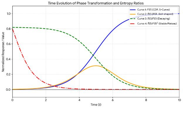
When the system exits this stable plateau, it means the control volume can no longer sustain a balanced rate of defect generation. Thermodynamically, this predicts exactly when the material will transition from highly organized nano-bands to coarser, irregular macro-grains. Engineers can use the boundaries of this specific plateau to calculate the maximum permissible processing time or thickness of a uniform nanostructured deposit before the material properties begin to degrade. Or it can predict more fundamental changes, such as a shift from Brownian motion to a different organized structure, as discussed below. The integrated entropy generation is always bounded.
Article Source. This is the first article to show how entropy generation is channeled into heat and stored work (stored energy) to choose a path of maximum entropy-generation rate, and to provide both classical and statistical descriptions. Examples include solidification, recovery, recrystallization, grain growth, sintering, and many biological transformations (activities). This course also covers connectivity and resilience, as described by S-curve transformations.
Core Concepts of Irreversible Entropy-Generating Processes.
- The Control Volume (CV): A specific region of interest where energy, mass, and entropy are reorganized to create new structural patterns or sub-boundaries.
- Maximum Entropy Production Rate (MEPR): This principle suggests that systems naturally select pathways during rapid changes—such as a supercooled liquid metal turning into a solid—by maximizing their rate of entropy generation per volume. [
- Internal Energy Redistribution: Entropy generation links directly to how internal energy is stored or transformed, whether as thermal shifts or structural “stored work” and “anti-work”.
- Boundary Defects: When new patterns emerge, they are stabilized by boundary defects (such as wear debris or high-entropy chemical concentration zones) that regulate the export of entropy from the system.
- In the control volume framework for dynamically self-organizing systems, pathway selection arrival refers to the exact operational point where a system transitions into a new organized state, which is mathematically determined by a specific ratio profiling boundary selection.
- This framework transitions the system from arbitrary variations into a definitive structural geometry by mapping the relationship between energy dissipation and entropy generation.
- The concept of pathway selection addresses a fundamental question in non-equilibrium thermodynamics: When a system is driven far from equilibrium, how does it “choose” its next pattern?
- The Tipping Point or Trigger Mechanism: Systems undergoing rapid transformations—such as rapid solidification from a supercooled melt or high-stress mechanical deformations—often evolve along non-linear, sigmoidal (S-curve) paths. The tipping points often are seen when the entropy generation rate demand can be met by a entropy generating event.
- The Arrival Criteria: Arrival occurs when the system satisfies the Maximum Entropy Production Rate (MEPR) principle. At this critical juncture, the system maximizes its volumetric entropy production rate, locking into the specific morphological pathway that distributes internal energy the fastest. [
- Energy Splitting: At the moment of arrival, the product of the local temperature and the entropy density production rate stabilizes to a constant. The system splits its internal energy between thermal accumulation (heat) and structural change (“stored work” and “anti-work”).
Every self-organizing process that generates entropy must distribute its internal energy. Part of this energy goes into heat, while the rest becomes stored work or anti-work. Anti-work represents the portion of internal energy that a system far from equilibrium forcefully uses to construct and refine internal physical boundaries rather than letting it dissipate purely as thermal heat. To find the exact amount of storable anti-work, the model mathematically integrates the thermodynamic availability generated by the [PDF/(CDF)^2] ratio over the entire life cycle of the structural transformation.
The [PDF/(CDF)^2] functions as a morphological sorting mechanism. While the MEPR dictates which directional pathway a process follows, the [PDF/(CDF)^2] also sets the physical limits of the boundaries themselves. The mathematical ratio directly models the exact rate of local entropy generation and governs how structural sub-boundaries form within a control volume.
Morphological Limitations are Predictable
The value of this ratio defines the geometrical features of the system:
- High Ratio Value: Favors pathways dominated by volume and structural transformations (e.g., coarser grain sizes or broader, more stable macrostructures).
- Low Ratio Value: Favors pathways dominated by localized, highly dissipative microstructural refinements (e.g., highly complex, micro-dendritic patterns or dense localized defects).
System Balance: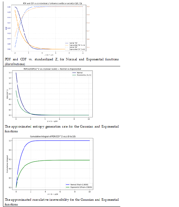
When new orders abruptly emerge, the pattern volume changes. The system balances the thermodynamic cost of building these physical boundaries against the rate at which it can export entropy. The ratio keeps the scale of generated shapes stable by matching internal energy storage to the emergence of localized boundary defects (such as high-entropy chemical segregations or physical phase separations).
The relationship between the [PDF/(CDF)^2] ratio and the Maximum Entropy Production Rate (MEPR) peak lies in the mathematical mapping of a dynamic transformation process. In the control-volume framework, the physical rate of volumetric entropy generation is directly proportional to this specific statistical ratio. Therefore, finding where this ratio reaches its maximum value identifies the exact physical location of the MEPR peak.
The MEPR peak determines the system’s final microstructure. If the transformation is highly compressed (a very sharp S-curve with a tiny standard deviation), the PDF becomes extremely tall and narrow.
This forces the [PDF/(CDF)^2] ratio to a much higher, more severe MEPR peak. Physically, a higher MEPR peak means the system injects a massive amount of “anti-Work” energy over a very short interval, resulting in highly refined, high-density boundary defects (such as ultra-fine grain sizes or dense dislocation networks).
The graph maps a standard Gaussian process to illustrate the pathway event for the Maximum Entropy Production Rate (MEPR) peak that takes over the control volume for a hypothetical transformation.

Notion of a tipping point and follow-on S-Curves
In the volume framework, anti-work represents the portion of internal energy that a system far from equilibrium forcefully uses to construct and refine internal physical boundaries rather than letting it dissipate purely as thermal heat. This allows for connectivity.
Storable Work: The instantaneous rate of storable anti-work generation—termed anti-power Wanti is directly coupled to the local volume VCV , a characteristic scaling temperature (T₀), and the volumetric entropy generation rate
Because the rate of entropy generation is proportional to the dynamic boundary selection ratio, the equation is written as:

Where:
- K is a system-specific thermodynamic coupling constant.
- VCV is the localized control volume.
- T₀ is the ambient or transformation temperature.
- z is the normalized process coordinate (such as time or position).
Because the Probability Density Function is fundamentally the derivative of the Cumulative Distribution Function: PDF(z) = d[CDF (z)]/dz, we can solve this integral analytically using a basic u-substitution.
Let u = CDF(z), so du = PDF(z). dz. And the calculation can be made to yield:

Note that the CDF term is related through its derivative to the rate (progression).
In fact, this is amazing because we can define u, its derivative, and its relationship to the entropy generation rate in a very broad way, and simple knowledge of an experimental transformation rate can yield a host of information.
An example that shows why this brilliant theory works, for example, in solidification:
Integrating the anti-work energy into structural physical dimensions reveals a direct link between thermodynamic variables, microstructural defects, and macroscopic mechanical strength. The energy stored per unit length of a single dislocation line is given by (E)~alpha G b^2. For pure copper:
-
- Shear modulus (G) = 48 GPa
- Burgers vector (b) = 0.256 nm
- Structural factor alpha = 0.5

Using Taylor’s Hardening Relation, where the Taylor factor (M) is (3.06), and the interaction coefficient (alpha^(prime)) is 0.3, this massive accumulation of defects restricts atomic slip planes. This theoretical input predicts a significant yield strength increase (note: Vickers Hardness Number is ~3x yield strength, MPa). While some of this energy is shared in real systems to form high-angle grain boundaries, treating it as a baseline upper limit translates to a noticeable spike in Vickers hardness, confirming why rapid solidification is such a powerful hardening mechanism. When reconfigured, one can use the Hall-Petch relationship for yield strength. To use the EGR/MEPR approach, we can choose the CDF progress for the cooling-rate difference as shown below. The Anti-work (i.e., the stored work that provides resilience after self-organization) is a function of the transformation rate.
| PARAMETER | RAPId Cooling (transformation) Path | Slower Cooling (transformation) Path |
|---|---|---|
| Initial Progress {CDF}(zi) | (0.01) (1%) | (0.05) (5%) |
| Final Progress {CDF}(zf) | (0.99) (99%) | (0.95) (95%) |
| Reciprocal Progress Factor
(see Anti-work vs CDF equation above) |
98.9 | 18.95 |
| Total Stored Anti-Work | 67.20 Joules | 12.86 Joules |
Physical implications of the example discussed above.
- Energy use differences for Anti-Work Transformation cause the total storable anti-work to decrease from 67.2 J down to 12.86J by slow transformation. This is fundamental to thermodynamics predictions from EGR and MEPR – namely, that a lower cooling rate yields a low-hardness metal alloy casting.
- Microstructure Structural Coarsening: Because the control volume has a much smaller energy budget to spend on building structural walls, it cannot support dense defect networks. Instead, when transformation energy is low, the system forms large, relaxed, coarse-grained structures with low mechanical hardness.
- A Nucleation Shock Concept: If a process initiates when progress is near zero {CDF}(zi) ~ 0, the denominator spikes dramatically. This proves that systems forced to transform rapidly from an un-nucleated state store (potentially) a massive amount of anti-work energy, forcing the creation of highly dense defects.
- Refinement of Microstructure: The total storable anti-work represents the exact energy budget available to generate physical surface area. The higher the calculated anti-work, the more physical sub-boundaries (finer grain sizes, denser dislocation walls) are formed, as the control volume is forced to construct itself in a manner to remain thermodynamically stable.
This approach is useful because it can handle discontinuous self-organization—abrupt transitions where a system switches from one geometric repetitive pattern to another (bifurcation).
| Material Process | Control Volume Boundaries | Active Irreversibility | Predicted Self-Organized Outcomes |
| Steady-State Solidification | Encloses the diffuse solid-liquid interface. | Solute diffusion gradients, latent heat dissipation, interfacial energy. | Transition from plane-front to cellular or dendritic arrays; primary arm spacing. |
| Friction & Wear Textures | Enclosed the sliding contact zone and sub-surface layer. | Plastic deformation, frictional heating, wear debris creation. | Self-assembled surface-texture patterns and localized defect densities. |
By calculating the total entropy generated for various geometrically possible states, the MEPR principle dictates that nature selects the configuration with the highest entropy production rate per unit volume as the dynamically stable path. This allows researchers to mathematically forecast critical thresholds—such as diffusion coefficients, exact supercooling limits where microstructure morphologies shift, cloud types, DNA machines, or reaction products.
Although it is well known that grain growth and sintering reduces the overall volume during grain growth the final volume does not equal the loss in grain boundary volume – its just short of that. The macroscopic volume contraction equals the ideal grain boundary volume loss minus the volume of newly generated lattice defects, elastic expansions, and residual triple junction anomalies that are a feature of entropy generation at a certain rate- just like in solidification.
Why is this analysis important for connectivity (from multiple follow-on S-curves or superimposed S-curves with varying features)? Can one think of life, or the difference between living and non-living things, based on the entropy generation rate? If you think about it, metabolic processes that are regulated by enzymes are just slow oxidation processes, albeit incredibly complex, information-guided optimization of chemical reaction rates when compared to rapid carbon oxidative processes like fossil fuel burning. Anti-work (and the battery-like storage ability it provides) is simply a way to sustain the critical cellular processes (work-enabled) required for life as we know it. Life can cease when anti-work is not adequate to sustain such processes, or when a different entropy-generation process cannot sustain normal cell replication. Instead of viewing life as a mystical exception to the laws of physics, modern thermodynamics treats living systems as highly efficient engines optimized to manipulate these rates.
What are some other phenomena where MEPR could be tested. Some examples where MEPR can be tested are: Magnetization of several common solid objects freshly introduced to a magnetic field causes dipoles to align and domains to grow. Such alignment and growth reduces the overall entropy and requires heat generation and body expansion (anti-work) to occur to compensate and conserve energy. MEPR could be tested for this effect! Or Can Anti-Work rate produce entropy generating black hole(s)? The fact that MEPR places bounds on the entropy rate generation rate is a huge clue here. Or for explaining the very unusual spin orientation of Uranus and her moons with respect to the orbital plane of our solar system.
Content created by JAS based on Source (link) and and related various references such as equilibrium and non-equilibrium clouds, solidification patterns (crystallization), bird organization during fight, and control volumes and wear.